The Mathematics of Electric Field Propulsion
To obtain the correct mathematical framework for an electrically isolated charged element we need to re-derive James Maxwell's equations from the potential of "Volts" and not from the "Magnetic Vector Potential" that James Maxwell used. This is simply done by multiplying the Magnetic Vector Potential by the speed of light or "c" (300,000,000 Meters/Second). We now get the following derivation shown below:
This derivation was first published in US Patent Application 20140009098. The derivation was done in this form so that an electrical engineer can understand it. This derivation is valid for charged objects in different inertial frames of reference or in the same inertial frame of reference. For charged objects in the same inertial frame of reference this derivation degenerates to the standard electrostatic equations with an added electric scalar potential. The Potential to Charge relation is an important element to this derivation that relates the charge on the object to its potential. In practice the capacitance is different for the different terms in this derivation. The reason is that the electric fields from these different potentials are in different inertial frames of references that cannot be shielded by electrostatic shielding in a significantly different inertial frame of reference. This is seen in the currently used electromagnetic framework as the inability of electrostatic shielding to shield a magnetic field. This effect creates disconnected electric field components in different inertial frames of references. The electric field intensities from these disconnected electric field components have to be calculated separately and then combined to get the correct total electric field. These new electric field components are seen as a magnetic field when an electric current flows in a wire conductor. These new components are now going to be defined as complex electric field components. The interaction of these new electric field components with static electric fields are the basis for propellant-less propulsion.
The Scalar Electric Potential Equation derives out as Volts/Meter but it's intensity is dependent on which inertial frame of reference that it is viewed from. So the derived Scalar Electric Potential Equation has to have the relative velocity difference taken into account to calculate it's intensity and correct units. From the stationary frame of reference the real units of this equation are seen as Volts/Second with the root scalar equation and it's intensity equation being the same equation. From the inertial frame of reference of the moving charged object it's intensity is "0".
The Scalar Electric Potential Equation derives out as Volts/Meter but it's intensity is dependent on which inertial frame of reference that it is viewed from. So the derived Scalar Electric Potential Equation has to have the relative velocity difference taken into account to calculate it's intensity and correct units. From the stationary frame of reference the real units of this equation are seen as Volts/Second with the root scalar equation and it's intensity equation being the same equation. From the inertial frame of reference of the moving charged object it's intensity is "0".
Now we have two equations instead of the three equations that we had in the old mathematical framework. The first equation is the "Electric Field Equation" with a new 2nd term. The last equation or the "Scalar Electric Potential Equation" that describes a new potential that is now is referenced to a point in space and will generate an electric field just like the potential from a charged object.
The first new electric field equation has the first and last term that is the same as the terms in the electric field equation being used today. The term on the right is the term that describes the electric field from the static electric charge. The term on the left tells us that a accelerating charge will generate an electric field from its acceleration. The term in the middle of the electric field equation of "DEL X (V/C) THETA" is new and its saying that when a charge is moving perpendicular to the observer, the observer will see an increase in the moving charges electric field. This middle term is describing the increase in the electric field of the Lorentz contracted charge that gives rise to the magnetic field when this charge is moving in a conductor.
This new middle term in our new electric field equation is represented as the magnetic field equation in the original electromagnetic derivation. This is the main reason that the current electromagnetic derivation is dependent on the characteristics of a conductor.
The new second equation is the "Electric Scalar Potential Equation". This equation is describing a new scalar or potential that forms at a point in space. This is different than the potential of a charged object where this potential is tied to the particles charge in the object and is known as a coupled charge. This new potential is different in that it is now coupled to a point in space instead of a charge. This new potential will now be seen as a decoupled electric field when viewed from a different inertial frame of reference than it was created in. This point in space has a the potential that can be built up to extremely large potentials over a specified time period. This is the reason that there is the time component (/seconds) in the units for this scalar. The real units for this scalar is really volts just like a coupled charge. The difference between the two types of potentials is that a coupled charge is fixed and cannot be built up over time (the electrons potential can never change over time) so there is no time component associated with a coupled potential. A decoupled charge can be built up over time so that it is always multiplied by the amount of time it took to build the scalar electric potential to give us our correct units of Volts. This term is the term that is the source of electromagnetic radiation except that there now is no "magnetic" in this type of radiation.
The last term or the term on the right of the Electric Scalar Potential equation is now a new potential that adds to or subtracts from a charged objects potential when it is approaching a point or receding from a point in space. This term effects the objects electric field by either increasing or decreasing an objects potential that the electric field is created from. So if a charged object with a potential of say 10 Kv is approaching a static electric field meter the field meter will see an electric field intensity that is from a charged object that has a potential that is more than 10 Kv . Then if the charged object is receding from the static electric field meter the meter will see an electric field intensity that is from a charged object that has a potential that is less than 10 Kv. This change in the potential is diagrammed below:
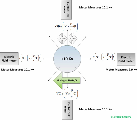
This diagram shows what a set of four identical static electric field meters would show if a moving charged sphere is measured by these meters when the sphere is equidistant to the meters. Mathematically the cross product is in the units of Volts/meter which is going to be different than the scalar potential which is in volts/second. This difference is more of an artifact of the mathematics indicating that the scalar potential has a connection to a point in space and the static electric field is connected to the charged object. To calculate the change in the electric field from the cross product of the velocity and the charge, the Del is taken of the static potential and added to the cross product of the velocity and charge. To get the change in the electric field from the dot product or electric scalar the potentials have to be added together and then the Del of the combined potential is taken to get the electric field. The time component "t " used in calculating the electric scalar potential in this example is the time it takes for 1/2 of the charged object to pass a point in space.
These electric field changes are very easy to measure from an electrically isolated charged object. These electric field changes are not seen from a charged conductive object that has a connection through a conductor to a high voltage power supply in a stationary inertial frame of reference. These electric field changes are only seen in isolated charged moving insulators or isolated conductors with no connections to a different inertial frame of reference. To correctly do this experiment the experimenter needs to use a charged element with the power source that is in the same inertial frame of reference as the object. A composite charged element that has a self contained battery and a high voltage boast module that is divided up into a + element and - element is the correct type of charged element to use for this experiment. Then the moving isolated composite object's electric field is measured by the electric field meters to see these relativistic electric field changes from the two different charged sections of the composite charged element.
There are a number of properties of the electric scalar that the mathematics are hinting at that can be exploited. The first one is that the electric scalar can be built up at a point in space. It turns out that if a moving charged object is accelerated perpendicular to its motion the leading or approaching scalar will not completely offset the trailing or receding electric scalar of the charged object. This effect is a direct result of the electric scalar potential being decoupled from the charge that created it. This effect is diagrammed below:
There are a number of properties of the electric scalar that the mathematics are hinting at that can be exploited. The first one is that the electric scalar can be built up at a point in space. It turns out that if a moving charged object is accelerated perpendicular to its motion the leading or approaching scalar will not completely offset the trailing or receding electric scalar of the charged object. This effect is a direct result of the electric scalar potential being decoupled from the charge that created it. This effect is diagrammed below:
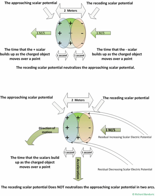
When a round positively charged non-conducting disk has a relative motion to an observer it will appear to have an approach and receding electric scalar potential that alters the disks electric field when observed in the direction of motion. As the charged non-conducting disk passes a point in space the leading scalar will increase as the front part of the disk passes over a point and then an offsetting trailing scalar will neutralize the change when the back half of the disk passes the same point.
This situation changes if the disk is accelerated perpendicular to its motion. Then the leading scalar is not going to be offset by the trailing scalar. Instead two scalar potentials are left behind the moving disk. The scalars that the disk leaves behind are curved channels that follows behind the edges of the disk.
In this example the two scalar channels will form and build up if the disk follows the same path by revolving about a point. The outer scalar channel will build up to a large positive potential. The inner scalar channel will build up to large negative potential.
This effect is seen when a charged non-conducting ring is rotated around its center of mass. A field meter measuring the rings outside potential will see the potential build up over time as the disk completes a number of revolutions.
The electric field changes that have been described by these new equations are easy to replicate and all that are needed to implement propellant-less propulsion.
The next question is why don't we see these effects reported?
We do and when they get reported they get disregarded and then rationalized to "another wacko!".
Lets look at these cases:
The next question is why don't we see these effects reported?
We do and when they get reported they get disregarded and then rationalized to "another wacko!".
Lets look at these cases: